Portable X‐Ray Fluorescence Spectrometry Analysis of Soils

Rationale For General Procedure

The elemental composition of soil is one of its most fundamental chemical parameters, affecting its reaction, salinity, cation‐exchange capacity (CEC), nutrient cycling, and pollutant transport. Early forays into soil chemical analysis relied on colorimetric wet chemistry methods such as titration or colorimetry [1]. In recent decades, these simplistic measurements gave way to methods offering greater accuracy and precision: atomic absorption spectrometry (AAS) and inductively coupled plasma atomic emission spectroscopy (ICP–AES). While the latter is the analytical standard for contemporary elemental analysis, both methods have some limitations; specifically, they require digestion of soil with caustic chemicals such as nitric or hydrochloric acids for partial digestion [2] or hydrofluoric acid for total digestion [3]. Therefore, these approaches require considerable time, energy, consumables, and laboratory‐based equipment.

By contrast, X‐ray fluorescence (XRF) was originally developed as a laboratory‐based technique [4], but it has since been miniaturized into small, portable units capable of making quality elemental determinations in situ with minimal sample preprocessing. The energies of most X‐rays reflect the core‐electron‐binding energies of atoms; thus, the atomic number strongly influences XRF effectiveness [5]. XRF describes the emission of fluorescent photons from a sample that has been irradiated by high-energy X-rays. As the emitted (fluorescent) secondary X-rays have discrete energies unique to a particular element and its local environment, X‐ray absorption (or emission) can be used for elemental determination in soils. Using the relationship between emission wavelength and atomic number, specific elements can be identified and quantified in a sample [6].

Early portable XRF (pXRF) instruments often featured radioactive isotopes as their excitation sources (e.g., Cd109 or Fe55) and featured Si‐PIN diode detectors [6]. In later generations, these radioactive isotope sources were replaced by miniaturized tube‐based X‐ray sources, and Si‐PIN diodes were replaced by silicon drift detectors, with the latter presenting tremendous advances in pXRF accuracy and precision. For purposes of discussion and methodology, all comments hereafter refer to experiences with an Olympus^® DELTA™ Premium (DP‐6000) pXRF configured with a 4 W Rh X‐ray tube operated at 10–40 keV.

Review of Existing Procedures

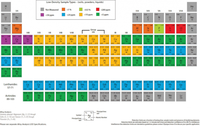
The use of pXRF for soil analysis offers many strengths relative to traditional laboratory‐based methods but also some limitations. One of the greatest advantages of pXRF is its field portability as it is configured as a handheld meter that can be taken to the field for in situ soil analysis. Scanning time varies widely but is typically in the order of ∼60 to 90 seconds. Longer scanning times (up to 300 seconds) increase the accuracy of elemental readings. Also, pXRF can be operated by rechargeable Li‐ion batteries, thus requiring no conventional electrical power supply on-site. Portable XRF offers a wide dynamic range of elemental quantification from low mg kg⁻¹ to high percentage levels, with no need for dilutions or restandardization. Lastly, pXRF analysis is multi‐elemental, providing simultaneous analysis of ∼20 elements. However, the detection limits of each element vary based on the atomic number and size of the electron cloud. Generally, elements with larger atomic numbers are measured more accurately than those with lower ones. For example, light elements such as P might have a limit of detection (LOD) of∼ ±5000 mg kg−1, whereas heavy elements such as U might have a LOD of ± 5 mg kg⁻¹ (Figure 1).

Despite numerous advantages, pXRF has several limitations. First, pXRF is variably affected by soil moisture. Literature points to a critical value of 20% moisture, a threshold above which drying or moisture correction should be considered. Weindorf et al. [7] noted that pXRF data quality was substantively reduced when evaluating frozen soils laden with ice relative to their dry counterparts.

Second, interelemental interferences are well documented. For example, As and Pb feature a shared spectral peak, making isolation and identification cumbersome [8]. Importantly, pXRF fails to distinguish elemental valence (e.g., Fe²⁺ vs. Fe³⁺) and merely reports total elemental concentration. Portable XRF also cannot read light elements (e.g., Z ≤ 11 Na). This is particularly limiting in soil analysis when the consideration of Na is important. However, some contemporary approaches have sought to overcome those limitations using other elemental data as proxies for the light elements of interest. In most pXRF instruments, the aperture through which X‐rays are emitted and fluorescence is detected is relatively small (∼2 cm). Applied to highly heterogeneous matrices in soils, results can vary dramatically over only a few lateral centimeters in a soil profile. Finally, pXRF lacks very low LODs (very low or high mg kg⁻¹) required for some investigations, where AAS or ICP–AES will remain the analytical standard for the foreseeable future.

Individual Steps in the Preferred Analysis, Including Justification

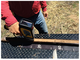
When conducting pXRF analysis of soil samples, several variables must be considered for optimal performance. First, the instrument must be properly standardized. The Olympus® DELTA™ pXRF features a calibration alloy clip (316 clip). Scanning the clip allows the instrument to lock into a standardized substance recognized by the integrated computer. Given the inherent heterogeneity in many soil samples, steps must be taken to ensure that pXRF scanning adequately reflects the composition of the soil being evaluated. When scanning in situ, the soil should be evaluated for concretions, nodules, or irregularities that may disproportionately affect pXRF performance; such areas should be avoided. The nose of the pXRF should be placed in direct contact with the soil, such that it makes good contact with a flat surface. In some instances, this may involve using a knife to gently scrape the soil to create a flat surface for scanning. To adequately capture variability within a given soil horizon, investigators should take multiple scans, physically repositioning the instrument between each scan to collect data on multiple points within a horizon. Excessive soil moisture (≥20%) denudes fluorescence received by the instrument [9]; thus, field evaluation of soil is best undertaken when soils are dry. In addition to scanning soil profiles, it can be convenient to scan soil cores collected with a hydraulic probe; the evaluation slot of the collection tube nicely accommodates the instrument's aperture (Figure 2). If field measurements are not essential, it may be preferable to scan soil samples ex situ after drying and grinding. Ex situ processing achieves two goals: reduction/elimination of soil moisture and sample homogenization. Scanning time is an important consideration as a longer scanning time produces optimized results. However, investigators must evaluate the need for reasonable sample throughput versus pXRF accuracy. Many soil evaluations typically use between 60 and 90 seconds for scanning [4]. A good practice for evaluating the quality of pXRF data is to scan the National Institute of Standards and Technology (NIST)-certified reference soil standards. A recovery percentage (pXRF determined/NIST-certified value) can then be calculated and reported with the pXRF data collected. Notably, pXRF tends to over- or underreport some elements, but many elements achieve results within 10% of NIST-certified values.

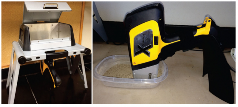
Although most instruments operate at low power (10–40 KeV), the operator must undergo proper radiation safety training to ensure safe operation as pXRF still produces ionizing radiation. The penetration depth of the X‐rays produced by pXRF instruments is commonly a few mm. Thus, exposing skin or body parts to X‐rays should be avoided. Furthermore, many states have licensing requirements for the use of radiation-producing devices that sometimes require the operator to wear a dosimetry badge to monitor X‐ray exposure levels. Leakage of X‐rays, which can be detected with a Geiger counter, most commonly occurs near the instrument's aperture if it fails to make planar contact with the sample being scanned. For comfort in prolonged use or specialized scanning applications, a bipod or sample stage can be used to position the pXRF for hands‐free operation (Figure 3).

Data Quality and Processing

Portable XRF for in‐field environmental studies has repeatedly proven useful for directly predicting metal concentrations in soil. For example, Radu and Diamond [10] reported strong coefficients of determination (R2) for Pb (0.99), As (0.99), Cu (0.95), and Zn (0.84) between pXRF and AAS. Furthermore, pXRF has shown potential for environmental quality assessment of peri‐urban agriculture, exhibiting reasonably strong correlations with ICP results of several trace elements [11]. However, pXRF elemental data can also be used as a proxy for predicting other soil properties.

Traditionally, scientists have utilized simple linear regression (SLR) and multiple linear regression (MLR) for establishing correlations between pXRF measured elements and physicochemical soil properties measured via standard laboratory procedures. For example, Sharma et al. [12] used pXRF for pH determination using elemental data as a proxy for soil pH. They used SLR and MLR to develop models associating pure elemental data from pXRF and pXRF elemental data with auxiliary input data (clay content, sand content, organic matter content). While MLR with auxiliary input data produced the best predictive model (R2 = 0.82; RMSE = 0.541), MLR with pure pXRF elemental data provided a reasonable predictability (R2 = 0.77; RMSE = 0.685). Notably, SLR could not produce a robust predictive model. Several other studies also included the development of SLR and/or MLR models (with or without auxiliary input data) to predict and find correlations between pXRF elemental data and traditionally lab-measured soil properties, such as soil CEC [13], soil salinity (electrical conductivity) [14], and soil gypsum content [15]. In all cases, the model(s) produced at least acceptable R2 values, ranging from 0.83 to 0.95 (see the full article for a complete reference list and detailed description of the studies). 

Both SLR and MLR are commonly used techniques relating pXRF elemental data to standard laboratory characterization data for the physicochemical parameters of interest. We recommend splitting the datasets into modeling (∼70%) and validation (∼30%) datasets when constructing a predictive model to assess model performance before using on unknown samples.

Recommendations

For common soil studies, ex situ scanning in the laboratory after drying and grinding of soil samples is preferable as this eliminates potential interference from soil moisture and provides increased sample homogeneity. As a balance between analytical accuracy and sufficient sample processing throughput, a scanning time of ∼60 to 90 seconds is recommended for most soil applications. However, if lower LODs are essential, extending the scanning time can optimize pXRF performance. The Olympus® DELTA™ pXRF features several modes for analysis (Soil, Geochem, Mining, Alloy). These modes offer different packages of elements used in various applications. For most common soil science applications, Soil mode works quite well. More exotic studies of pollution sources or mine soil tailings may benefit from Mining or Alloy modes. In some instances, scanning with more than one mode can be useful, where certain elements are reported more accurately by one mode than another. These modes use various energies and filters to produce fluorescence signatures of various elements. The use of specialized filters may also enhance instrument performance for certain applications in which background scatter or interference can be isolated, allowing better performance [16].

Sample Applications and Case Studies, Including Calculations

To date, pXRF has been used to quantify elemental concentrations in several media [4]. While early pXRF studies focused on geologic, metallurgical, or archeological uses, newer soil science and agronomy applications have developed rapidly in recent years. Portable XRF is a good method for use in instances where the chemical properties of soils are of importance. Portable XRF will not provide LODs as low as traditional ICP–AES or ICP–MS analysis. Portable XRF reports total elemental concentration in soils, while techniques such as ICP–AES depend on the success of the digestion used to extract elements into solution. However, pXRF can provide in situ data of reasonable accuracy, with minimal to no sample preparation in ∼60 to 90 seconds. Also, pXRF may be useful in certain specialized applications where nondestructive analysis is required or matrices that do not lend themselves readily to traditional soil physicochemical analysis. Similar to spectral data collected by visible and near-infrared (VisNIR) spectroscopy, once collected, pXRF elemental data can be used to predict many physicochemical soil parameters. Universal predictive models can be used with some degree of accuracy, but for optimal results, it is advisable to collect pXRF elemental data, process the soil samples by traditional laboratory analysis, and then develop customized predictive models for a given area. In most cases, a customized model will show considerable accuracy across a given region as long as the general geological and soil properties remain similar. Importantly, the samples used in constructing the model should reflect the variability the investigator seeks to directly predict from the pXRF data. For example, if two substantively different soils are studied, two different models should be developed.

Most models are built on MLR, using elemental data as proxies for the parameter of interest. In developing the predictive model, the investigator should collect a robust dataset (n ≥ 100 or more), reflective of all variability likely to be encountered in future analysis with the model. Randomly, 30% of the samples should be removed from the dataset for independent validation, with 70% of the samples used for model calibration. Calibration performances can be observed in terms of R2, RMSE, bias, residual prediction deviation, and ratio of performance to inter‐quartile range. 

Alternatively, concatenating pXRF elemental data with spectral data from other proximal sensors like visible VisNIR diffuse reflectance spectroscopy can be used in advanced algorithms like penalized spline regression (PSR), partial least squares regression, and random forest regression (RF) to predict several soil parameters with high accuracy [17]. The addition of remote sensing data has also been shown to increase model prediction accuracy [18]. Besides, an advanced combined modeling approach (PSR + RF) can be used in which PSR is used to fit the training set (containing VisNIR spectra only) using full cross‐validation to choose the tuning parameter. Next, RF can be used to fit the residuals of the PSR model on the PXRF elemental data. The final predicted value represents the combination of PSR and RF predicted values [19].

Original Article:

Weindorf, DC,  Chakraborty, S.  Portable X-ray fluorescence spectrometry analysis of soils. Soil Sci Soc Am J.  2020; 84: 1384– 1392. https://doi.org/10.1002/saj2.20151

References

[1] C. B. Fliermans, T. D. Brock, Soil Science 1973, 115, 120.

[2] USEPA, Method 3050B: Acid digestion of sediments, sludges, and soils, 1996, www.epa.gov.

[3] USEPA, Method 3052: Microwave assisted acid digestion of siliceous and organically based matrices, 1996, www.epa.gov.

[4] D. C. Weindorf, N. Bakr, Y. Zhu, Adv. Agron. 2014, 128, 1. 

[5] W. P. Gates, in Handbook of clay science, Elsevier, New York, 2006.

[6] D. J. Kalnicky, R. Singhvi, J. Hazard. Mat. 2001, 83, 93.

[7] D. C. Weindorf, N. Bakr, Y. Zhu, A. McWhirt, A., C. L. Ping, G. Michaelson, C. Nelson, K. Shook, S. Nuss, Pedosphere 2014, 24, 1.

[8] A. Whirt, C. D. Weindorf, Y. Zhu, Compost Sci. Util. 2012, 20, 185.

[9] S. Piorek, in Current protocols in field analytical chemistry, John Wiley & Sons, New York, 1998.

[10] T. Radu, D. Diamond, J. Hazard. Mater. 2009, 171, 1168.

[11] D. C. Weindorf, Y. Zhu, S. Chakraborty, N. Bakr, B. Huang, Environ. Monit. Assess. 2012, 184, 217.

[12] A. Sharma, D. C. Weindorf, T. Man, A. Aldabaa, S. Chakraborty, Geoderma 2014, 232–234, 141.

[13] A. Sharma, D.C. Weindorf, D. D. Wang, S. Chakraborty, Geoderma 2015, 239–240, 130.

[14] S. Swanhart, D. C. Weindorf, S. Chakraborty, N. Bakr, Y. Zhu, C. Nelson, K. Shook, A. Acree, Soil Science 2014, 179, 417.

[15] D. C. Weindorf, J. Herrero, C. Castañeda, N. Bakr, S. Swanhart, Soil Sci. Soc. Am. J. 2013, 77, 2071.

[16] S. Bichlmeier, K. Janssens, J. Heckel, D. Gibson, P. Hoffmann, H. M. Ortner, X‐Ray Spectrom. 2001, 30, 8.

[17] D. D. Wang, S. Chakraborty, D. C. Weindorf, B. Li, A. Sharma, S. Paul, M. N. Ali, Geoderma 2015, 243–244, 157.

[18] A. A. A. Aldabaa, D. C. Weindorf, S. Chakraborty, A. Sharma, Geoderma 2015, 239–240, 34.

[19] S. Chakraborty, D. C. Weindorf, B. Li, A. A. A. Aldabaa, R. K. Ghosh, S. Paul, M. N. Ali, Sci. Total Environ. 2015, 514, 399.