A New Method of Imaging Particle Tracks in Solid-state Nuclear Track Detectors

Methods

Aim

The aim of this study was to acquire and analyze high-resolution 2D and 3D image data of etched radon tracks in CR-39 detectors.

Material and methods

A LEXT OLS3100 confocal laser scanning microscope (Olympus Corporation, Japan) with a 408 nm laser was used in order to acquire images of four etched CR-39 radon detectors. In this study, two objective lenses (50X and 100X) were used for the collection of 3D data, both having a numerical aperture of 0.95. The manufacturer’s user manual (version 5) indicates that the microscope has a planar resolution of up to 0.12 μm (using the 100X objective) and a height resolution of up to 0.01 μm. The detectors from the Radon Metrology Laboratory at Kingston University were put on a glass slide, which was then placed on the microscope stage.

Acquisition and analysis of 2D surface images

In this study, 2D surface images of the detectors, obtained with a 10X objective, were analyzed. With the 10X objective lens, each pixel corresponded to 1.25 μm. A charge-coupled device is used to acquire 2D color images from reflected light. The maximum number of pixels per field of view using the charge-coupled device camera (optical) is 1024 x 768. Images of the central portion of the detectors were processed using software we developed at Kingston University using MATLAB (The MathWorks, Inc., Natick, MA, U.S.A.). The color images (.bmp files) were converted to gray scale and then binary following manual entry of an appropriate threshold value; using the software small objects in the resultant binary image were removed and a 3 x 3 median filter was applied. Appropriate detection of the radon tracks could be checked from an image obtained by superimposing a contour of the detected tracks onto the gray scale or color image, and hence, the suitability of the threshold could be visually assessed. Tracks near the edge of the image were not included in case they were not complete. The detected objects were then analyzed using the ‘regionprops’ function in MATLAB; this method is similar to that previously described[9]. The area, perimeter, and shape of the tracks were assessed. In addition, the images were visually examined in order to investigate the possible occurrence of closely spaced tracks. Tracks were identified visually on the light white background as dark round or elliptically shaped objects that may have a pale center.

Acquisition and analysis of 3D images

The LEXT microscope was used in confocal mode in order to acquire 3D image data of more than 60 tracks of which 51 were single tracks. The height of the top surface and the deepest track were manually determined in order to allow the image data to be acquired over an appropriate depth range. For this study, a 50X objective was used for the initial 3D examination of the detectors as this appeared to give an appropriate level of detail for the tracks while allowing several tracks to be imaged. The movement between each step in the z-direction was 180 nm for the 50X objective and 50 nm for the 100X objective. For the 50X objective lens, each pixel corresponds to 0.25 μm. In order to view further surrounding tracks, the tiling feature was used to acquire a series of adjacent images which were then stitched together; the stitching involves a 15% overlap of the adjacent tiled images. The 3D visualizations were compared with 2D surface images.

The 3D data, including height information, was visualized and analyzed using the LEXT system. Hence the depth profile and changes in gray level were examined in tracks that appeared to be inclined, as identified by an elliptical cross-section, by manually selecting cross-sections through the visualization of the tracks. We also investigated possible connections between tracks when there were closely spaced multiple events. Data with height information was also exported to a spreadsheet-compatible file so that it could be visualized with additional software we developed using MATLAB.

Results

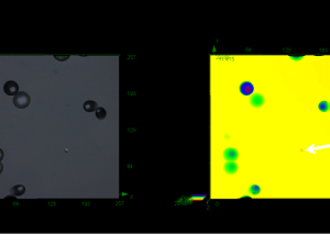
A total of 229 single tracks or clusters of multiple tracks (range 53 to 63 per detector) were seen in the images of the four detectors. An example of an image of tracks and their detection is shown in Figure 1. There were 182 clear single tracks, 25 double adjacent tracks, and 7 regions of apparently more than 2 adjacent tracks; there were a further 15 single or double tracks where there appeared to be some artifacts and hence were not included in the following analysis. The area data for the single tracks was not consistent with a normal distribution using the Ryan–Joiner test in MINITAB v. 15 (Minitab, Inc. State College, PA, U.S.A.), and hence median, quartiles, and range are used for the descriptive statistics. The area, perimeter, equivalent diameter, roundness, and eccentricity of the single and double radon tracks are shown in Table 1.

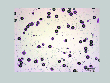
Table 1: Table 1: Minimum, Q1, median, Q3, and maximum values of area, perimeter, roundness, and other measures for single and double tracks.

Eccentricity is the ratio of the distance between the foci of the ellipse divided by the length of the major axis; thus, for a circle the value is 0. The eccentricity values suggest that most of the single tracks are elliptical, which is consistent with visual observation. Using Spearman’s rank correlation there is a significant negative correlation between area and eccentricity (r 0.541, n 182, P < 0.001), although there was wide variation when examining the data with a scatter plot.

Compactness is defined as the ratio of perimeter squared divided by area[15] and roundness is that ratio divided by 4π[16]. Thus, a circle has the lowest roundness of 1. In this data, all the objects had a roundness of 1 or more except for one very small object (222 pixels in area) with a measured roundness value of 0.97. The median roundness of the single tracks of 1.09 is also consistent with many tracks not being exactly circular in cross-section.

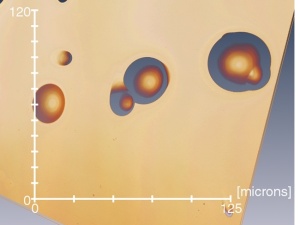
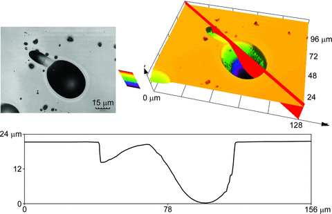
Three-dimensional visualization helps in investigating variation in area and depth as well as identifying coalescing tracks as seen in Figure 2 where a 50X objective was used. The examples in Figures 2 and 3 show that track areas appear to be highest at the surface and become smaller going deeper into the detector. The 3D image data in Figure 2 was exported to a spreadsheet file in order to enable the analysis of the track area using additional software developed using MATLAB (The MathWorks, Inc.) at Kingston University. The software detects the surface layer and hence can identify tracks emanating down from the top surface. From the 3D image data, the area of nine single tracks at the detector surface was analyzed and compared with a corresponding 2D image acquired with a 10X objective. The mean (standard deviation) difference in the track area, (3D – 2D measurements) divided by the mean of the 2D and 3D area, was 5.1% (4.2%); this data was consistent with a normal distribution using the Ryan–Joiner test in MINITAB v. 15 (Minitab, Inc.) and using a one-sample t-test were significantly different from 0 (P = 0.008).

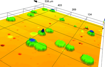
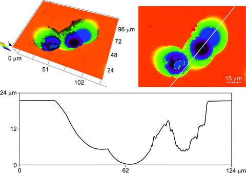
Acquisition of each 3D dataset (without tiling) takes typically about 5 minutes depending on settings; 130 steps can be scanned per minute in the z-direction when using any of the objectives. Visualization and basic analysis of the 3D track data typically takes less than 10 minutes, depending on the size of the image and the type of analyses performed. Some of the observed elliptical shape tracks were associated with different gradients on either side of the corresponding depth profile of the 3D data. From the profile graph in Figure 3, the deeper track can be seen to have a depth of about 22 μm whereas the shallow track has a depth of about 10 μm. An indication of the track angle can be derived from the depth and spatial position data. The gradient of the profile is likely to indicate the angle at which the α particle hit the detector; two examples of this are seen in Figures 3 and 4, which also show that 3D visualization and depth profiles can help in understanding the relative size and angles of a sequence of multiple hits from the way in which the tracks are formed (Figure 4). The profile graph in Figure 4 shows clearly the depths of the two tracks on the right are about 18 and 22 μm. In addition, in the example in Figure 4, the outline 2D shape suggests there may be two tracks, whereas the greater detail from 3D visualization shows that there are three tracks.

Discussion

In this study, clear visualizations of surface and 3D tracks were obtained and a number of patterns such as single, double, and multiple hits as well as angled hits were observed. Further to our earlier paper[9], in this investigation, 3D images of the full depth of tracks together with greater detail were obtained. The lower wavelength laser as well as the 50X and 100X objective lenses used here for 3D microscopy contribute to the improved resolution. Hence, it was possible to visualize in detail the occurrence of angled tracks in 3D and to quantify the angle along different profile lines; such visualization allows assessment of the direction in which the α particles collide with the detector. From the 2D image data, the area of tracks shows marked variation, and preliminary results suggest that this may be inversely related to the eccentricity, which is consistent with visual observations that lower area tracks appeared to be more elliptical in shape. It would be interesting to investigate if area is related to the angle of inclination. The 50X objective used for 3D dataset collection enables higher spatial resolution images than the 10X objective and hence correspondingly influences track area measurement accuracy. Measurements of surface track area obtained from a 3D image using the 50X objective were found to be similar to corresponding area measurements from a 2D image using the 10X objective; the mean difference observed was 5.1% which, albeit small, was significantly different from 0 (P = 0.008). The higher track area, observed using 3D imaging, is likely to be due to the decrease in the area seen going deeper into the detector. For 2D imaging, this may result in less contrast around the circumference of the track, which thus could affect the area detected when applying the thresholding algorithm.

The variability of radon track measurements from 2D measurements may in part be due to the difficulty of selecting true tracks from an artifact. It was observed that high-resolution 3D visualization can help in accurately identifying tracks and quantification of their geometry. Although collecting 3D datasets takes more time than conventional 2D imaging, the 3D data enables further analysis of tracks than from 2D data alone; this should help in better understanding track formation and more precise determination of the number of radon tracks. For example, multiple closely spaced tracks could be due to hits from multiple particles or possibly bouncing of particles on the detector surface; 3D imaging should enable the distinction of particle bouncing from multiple particle hits by assessment of the depth and angle data. The occurrence of areas of adjacent multiple hit tracks was observed; the reason for α particles appearing to impinge on the detector more often in certain areas is unclear, but it is possible that the process of track formation causes a change in surface charge. In summary, high-resolution 3D images of radon tracks in CR-39 plastic detectors obtained using confocal microscopy in combination with 2D microscope images enable detailed analysis of their physical dimensions and shape; the full depth of tracks and their angle with respect to the surface could be quantified. The techniques described in this study allow detection of tracks of different sizes and may thus help to improve the accuracy and repeatability of radon measurements as well as gain a better understanding of track formation.

References

[1] Darby, S., Hill, D., Auvinen, A., et al. (2005) Radon in homes and risk of lung cancer: collaborative analysis of individual data from 13 European case-control studies. BMJ. 330, 223–226.

[2] ICRP (International Commission on Radiological Protection) (2007) Recommendations of the International Commission on Radiological Protection. ICRP publication 103. Ann. ICRP. 37(2–4), 1–332.

[3] Papworth, D.S. (1997) A need to reduce the radon gas hazard in the UK.

J. R. Soc. Health. 117, 75–80.

[4] Coskeran, T., Denman, A., Phillips, P., Gillmore, G. & Tornberg, R. (2006) A new methodology for cost-effectiveness studies of domestic radon remediation programmes: quality-adjusted life-years gained within primary care trusts in Central England. Sci. Total Environ. 366, 32– 46.

[5] Gillmore, G.K., Phillips, P., Denman, A., Sperrin, M. & Pearce, G. (2001) Radon levels in abandoned metalliferous mines, devon, Southwest England, Ecotoxicol. Environ. Saf. 49, 281–292.

[6] Gillmore, G., Gilbertson, D., Grattan, J. et al. (2005) The potential risk from radon222 posed to archaeologists and earth scientists: reconnaissance study of radon concentrations, excavations and archaeological shelters in the Great Cave of Niah, Sarawak, Malaysia. Ecotoxicol. Environ. Saf. 60, 213–227.

[7] Phillips, P.S., Denman, A.R., Crockett, R.G.M., Gillmore, G., Groves- Kirkby, C.J. & Woolridge, A. (2004) Comparative Analysis of Weekly vs. Three Monthly Radon Measurements in Dwellings. DEFRA Report No., DEFRA/RAS/03.006. DEFRA, London.

[8] Cliff, K. & Gillmore, G.K. (eds.) (2001) The radon manual: a guide to the requirements for the detection and measurement of natural radon levels. Associated Remedial Measures and Subsequent Monitoring of Results, 3rd edn. The Radon Council, Shepperton, Middlesex, U.K.

[9] Petford, N., Wertheim, D. & Miller J.A. (2005) Radon track imaging in CR-39 plastic detectors using confocal scanning laser microscopy. J. Microsc. 217, 179–183.

[10] Naismith, S.P., Howarth, C.B. & Miles, J.H.C. (1998) Results of the 1997 European Commission Intercomparison of Passive Detectors. EUR 18035 EN. European Commission, Brussels.

[11] Henshaw, D.L., Allen, J.E., Keitch, P.A. & Randle, P.H. (1994) Spatial distribution of naturally occurring 210Po and 226Ra in children’s teeth. Int. J. Radiat Biol. 66, 815–826.

[12] Nikezic, D. & Yu K.N. (2008) Computer program TRACK_VISION for simulating optical appearance of etched tracks in CR-39 nuclear track detectors. Comput. Phys. Comm. 178, 591–595.

[13] Wagner, W. & Van Der Haute, P. (1992) Fission Track Dating. Kluwer Academic Publishers, Dordecht.

[14] Fleischer, R.L., Price, P.B. & Walker, R.M. (1975) Nuclear Tracks in Solids: Principles and Applications. University of California Press, Berkley, California.

[15] Gonzalez, R.C. & Woods, R.E. (2002) Digital Image Processing, Second edn, Prentice Hall, New Jersey.

[16] Kanthathas, K., Willmot, D.R. & Benson, P.E. (2005) Differentiation of developmental and post-orthodontic white lesions using image analysis. Eur. J. Orthod. 27, 167–172.

Copyright:

10.1111/j.1365-2818.2009.03314.x

D. Wertheim, G. Gillmore, L. Brown, N. Petford;

Journal of Microscopy;

© 2009 Crown Copyright Journal compilation

© 2009 The Royal Microscopical Society