Application of Confocal Microscopy for Surface and Volume Imaging of Solid-state Nuclear Track Detectors
Background
As outlined in this article digest, the inhalation of radon gas has been shown to be a risk factor in the development of lung cancer[1]. It is estimated that there are 1,100 home radon-related lung cancer deaths annually in the United Kingdom alone[2]. Radon levels can be measured using small etched plastic detectors called solid-state nuclear track detectors (SSNTDs); the detectors are often based on poly-allyl-diglycol carbonate or PADC, commercially known as CR-39.
CR-39 detectors
SSNTDs are more similar to human tissue than other passive detectors[3]. They are extensively used in dosimetry because of their low linear energy transfer (LET) threshold for detection of charged particles[4], hence their use in measuring radon and its decay products in buildings. SSNTDs are also used in neutron dosimetry and the neutron response of such detectors has relied on the simulation of the formation/development of etched tracks as a function of energy and etching time[5]. Some authors have undertaken simulated 3D computation of track shape in order to better understand the potential effect of incidence direction of charged particles and SSNTD track development[6,7]. The measurement of track parameters then can provide data on the energy deposition of the incident particle[3], and analysis of tracks produced by α particles, protons, or nuclear fission fragments is a very valuable tool[8]. The geometry of α-track cone formation in SSNTDs can provide information on energy and charge and direct measurements of track lengths are sometimes required[8]. The α-track etch-pit diameters can act as a spectrometer in that they can be related to incident α energy[9]. In one study, detectors were broken in order to make direct measurements of the track length[7], while others have utilized atomic force microscopy (AFM), but due to probe geometry the bottom of the track has not been reached[8]; a holographic technique in combination with an interferometer has also been applied to obtain surface views of tracks[8]. Thus, there have been few studies imaging actual track depths using nondestructive techniques.
SSNTD imaging
Conventionally etched SSNTDs are assessed using 2D microscope imaging. Confocal microscopy can be used to obtain 3D image datasets of tracks in SSNTDs[10,11]. Fluorescent confocal microscopy was used to image SSNTDs by treating the detectors with Nile Blue A[10]. We have previously used the LEXT™ OLS3100 confocal microscope to successfully image CR-39 radon track detectors[11-13]. These studies used reflection confocal microscopy to enable 3D visualization and quantification of tracks from surface data without the need for using a fluorescent dye. A recent addition to the LEXT™ OLS4000 microscope enables z-stack images to be stored in addition to the acquisition of surface image data. Hence, this potentially allows examination of 3D material structure around tracks which may help in the interpretation of coalescing and angled tracks.
Aim
The aim of this study was to investigate single and coalescing particle tracks with surface and volume visualization of confocal microscope SSNTD image datasets.
Method
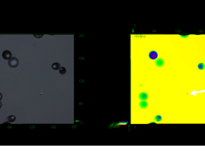
Nine CR-39 plastic radon detectors previously exposed in rooms, or a controlled radon chamber were processed by etching for up to 4.5 hours in 6M NaOH solution at 90 °C (194 °F) in the KU (Micro) Radon Laboratory at Kingston University; the etching conditions could potentially affect the microscopic appearance of tracks. The etched SSNTDs were cleaned with distilled water in an ultrasonic bath for 2 minutes. Detectors were individually placed on the microscope stage of an Olympus LEXT™ OLS4000 confocal microscope (Olympus Corporation, Japan). The microscope system was equipped with the Olympus LEXT Remote Development Kit (RDK), thus allowing acquisition of z-stack images as well as surface imaging. The detectors were initially examined using the LEXT operating in 2D imaging mode using 5X and 10X objective lenses followed by 3D scanning using the standard ‘fine’ surface scanning mode (with ‘Color’); the method is similar to that used in earlier studies with an OLS3100 microscope[12,13]. In confocal mode, 50X or 100X objective lenses were used (NA 0.95), and the microscope has a 405 nm laser. The images were acquired with a size of 1024 × 1024 pixels; using the 50X lens, the xy area imaged was 260 × 260 μm, thus giving a lateral spatial resolution of 0.25 μm per pixel. Before scanning, the top (upper detector surface) and bottom levels were determined manually. 2D and 3D screenshots were acquired as single image files. Heightmap data were downloaded in a spreadsheet-compatible file in order to allow subsequent 3D visualization and analysis.
In this study, we examined and compared surface data with z-stack imaging. The surface data were analyzed from the heightmap spreadsheets. Z-stack imaging was obtained using the LEXT RDK, and hence it is possible to enable volume visualization from the confocal slices.
Script files were written for the RDK to run on the controlling PC in order to allow appropriate movement of the objective lens following each z-slice acquisition; in each script file, movement was set such that the objective lens moved up away from the slide in 0.1 μm steps. As the top and bottom positions were known, the number of slices to be acquired could be calculated, and hence the number of slices to be collected was set in the script file; the z-stack images were collected.
3D visualization
Software was written in MATLAB (The MathWorks Inc., Natick, MA, U.S.A.) in order to read the height field map spreadsheet files. The mode height was calculated to determine the level of the detector surface. The minimum and maximum heights were computed, and the data was remapped as a gray scale image covering the full range of height values. The resultant images were read into Amira v. 5.4 (VSG, Visualization Sciences Group), and networks were developed to allow examination of the 3D visualization. Further software was developed in MATLAB in order to display surface data and compute the distribution of track depths.
Surface and volume visualizations of the z-stack images were also performed using Amira; isosurface and voltex visualization techniques were applied to examine the image data.
Comparison of track depths
Track depths calculated from the surface spreadsheet files were compared with the stack data for 45 tracks in the nine detectors. In Amira, the depth of the tracks was examined using orthoslice visualization; in this mode, the signal from the confocal microscope imaging can easily be seen in successive z-slice images, and an example can be seen in Figure 1C. The track depths were thus calculated from the difference between the detector surface level and the lower surface of each of the tracks as the distance between slices is constant; the lower surface was defined as the lowest position where the track is discernible. Data were tested for consistency with a normal distribution using the Ryan–Joiner test in Minitab v. 16 (Minitab Inc., U.S.A.).
Results
Visualization using 3D surface and volume approaches were compared. Figure 1 shows an example of surface imaging from depth data in comparison with volume visualization. The Figure shows views from the lower side of the detector and looking from the top surface. This is compared with volume visualization (Figure 1D) formed by combining the z-stack of intensity images, one of which is shown in Figure 1C. The techniques applied for volume visualization of the stack data did not apply connection of surfaces so that the raw intensity data were used; this can result in apparent gaps but avoids potential difficulties from applying assumptions about surface geometry.
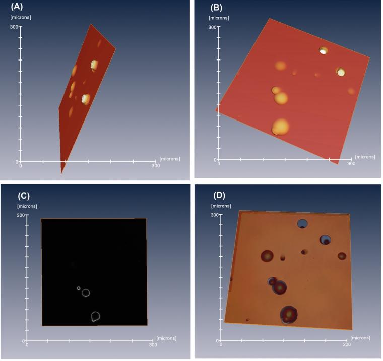
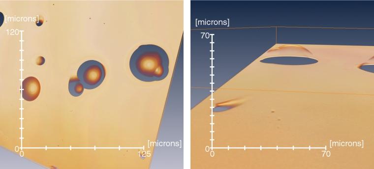
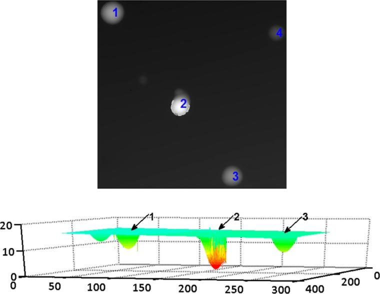
Figure 2 shows an example of zooming in on an angled track as well as two apparently very closely coalescing tracks. The volume visualization technique allows zooming in to examine the surface in more detail, thus identifying the likely closely coalescing tracks and the appearance of an angled track. These examples illustrate that visualization of z-stack data enables structure of the tracks deep in the detector to be seen. An example of the analysis of track depth data using software we developed in MATLAB is shown in Figure 3. Using data from another detector, the representation of depth in a gray scale or pseudocolor image helps to assess the depth of each individual track with respect to the detector surface. Tracks 1, 2, and 3 have depths of 7.5, 14.5, and 6.6 μm, respectively, as can be seen in the lower part of the figure with a 3D representation obtained using software we developed in MATLAB.
Comparison of track depths
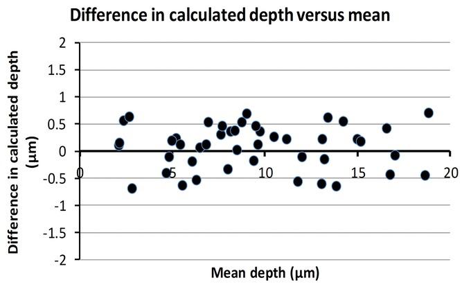
The mean (standard deviation) depth of the 45 tracks was 9.5 (4.6) μm. Figure 4 shows a graph of the difference in calculated depth (surface depth minus stack measured depth) against the mean in accordance with a method for comparing measurements[14]. The mean (standard deviation) difference in calculated depths between the two methods was 0.08 (0.40) μm. There was no significant correlation between the difference in the two measurements and the mean (Pearson’s correlation coefficient r = −0.02, p = 0.9). The depths are consistent with previous observations[13].
Discussion
Assessment accuracy is important not only for radon detection and remediation but also for dosimetry. Coalescing tracks may cause problems of interpretation using conventional 2D analysis, these difficulties could be addressed using 3D imaging which also helps to distinguish real tracks from artifacts; artifacts due to dust or similar particles should be evident by protrusion above the top surface. Coalescing tracks are likely to be particularly evident with high track densities associated with high radon concentrations.
Detection of surface features has wide applications in material analysis. In the case of SSNTDs, surface tracking may be difficult for very steep tracks that could occur in some deep and angled tracks. Furthermore, coalescing tracks could be difficult to assess because of the associated complex profile. Z-stack imaging allows the raw data to be displayed, thus avoiding possible artifacts that may be seen in steep, angled tracks; furthermore, the method allows a detailed view of the structure of coalescing tracks. Hence, 3D imaging allows examination of coalescing tracks and helps to discern real tracks from artifacts, both of which potentially could be problematic in 2D analysis. The examples in Figures 1 and 2 illustrate that visualization of z-stack data images allows examination of the structure of tracks deep in the detector.
Rather than only imaging the surface, in transparent and partially transparent materials, stack imaging should allow examination around the surface into the material. Thus, we have been able to study the structural appearance of tracks. Additional information can possibly be obtained regarding surfaces associated with steep angles with respect to the upper surface. The stack imaging system enables examination of the reflected signal, thus allowing detailed interpretation of the data associated with steep angular features as can be seen, for example, in deep tracks and certain angled tracks. In addition, if 3D surface imaging identifies unexpected surfaces, stack imaging can help in the interpretation of data in order to understand better the resultant visualization. The comparison of calculated depths using the two techniques showed good agreement.
Conclusions
Series of z-stack images were acquired using the Olympus LEXT™ RDK as well as surface imaging data with the microscope and software was developed to enable 3D visualization and analysis of the data in order to examine radon tracks in CR-39 detectors. Stack imaging can enable visualization that complements conventional 3D surface imaging as it allows examination of the material surrounding the detected surfaces. Comparing the two analysis techniques, there was good agreement in the calculated measurement of track depth. This approach should enable the assessment of the structure of tracks deep in the detector, which could help in the interpretation of images and hence improve SSNTD assessment.
References
[1] Darby, S., Hill, D., Auvinen, A., et al. (2005) Radon in homes and risk of lung cancer: collaborative analysis of individual data from 13 European case-control studies. Br. Med. J. 330, 223–228.
[2] Gray, A., Read, S., McGale, P. & Darby, S. (2009) Lung cancer deaths from indoor radon and the cost effectiveness and potential of policies to reduce them. Br. Med. J. 338, 215–218.
[3] Caresana, M., Ferrarini, M., Fuerstner, M. & Mayer S. (2012) Determination of LET in PADC detectors through the measurement of track parameters. Nucl. Instr. Methods Phys. Res. A 683, 8–15.
[4] Lounis, Z., Djeffal, S., Morsli, K. & Allab, M. (2001) Track etch parameters in CR-39 detectors for proton and alpha particles in different energies. Nucl. Instr. Methods Phys. Res. B 179, 543–550.
[5] Do¨rschel, B., Bretscheider, R., Hermsdorf, D., Kadner, K. & Ku¨ hne, H. (1999) Measurement of the alpha track etch rates along proton and alpha particles trajectories in CR-39 and calculation of detection effi ciency. Rad. Measur. 31, 103–108.
[6] Azooz, A.A., Hermsdorf, D. & Al-Jubbori, M.A. (2013) New approach of modeling charged particles track development in CR-39 detectors. Rad. Measur. 58, 94–100.
[7] Do¨rschel, B., Hermsdorf, D., Reichelt, U., Starke, S. & Wang, Y. (2003) 3D computation of the shape of etched tracks in CR-39 for oblique particle incidence and comparison with experimental results. Rad. Measur. 37, 563–571.
[8] Palacios, F., Palacios Ferna´ndez, D., Ricardo, J., Palacios, G.F., Sajo-Bohus, L., Goncalves, E., Valin, J.L. & Monroy, F.A. (2011) 3D nuclear track analysis by digital holographic microscopy. Rad. Measur. 46, 98–103
[9] Soares, C.J., Alencar, I., Guedes, S., Takizawa, R.H., Smilgys, B. & Hadler, J.C. (2013) Alpha spectrometry study on LR115 and Makrofol through measurements of track diameter. Rad. Measur. 50, 246–248.
[10] Hermsdorf, D. & Hunger, M. (2009) Determination of track etch rates from wall profiles of particle tracks etched in direct and reversed direction in PADC CR-39 SSNTDs. Rad. Measur. 44, 766–774.
[11] Petford, N., Wertheim, D. & Miller, J. (2005) Radon track imaging in CR-39 plastic detectors using confocal scanning laser microscopy. J. Microsc. 217, 279–283.
[12] Wertheim, D., Gillmore, G., Brown, L. & Petford, N. (2010a) A new method of imaging particle tracks in Solid State Nuclear Track Detectors. J. Microsc. 237, 1–6.
[13] Wertheim, D., Gillmore, G., Brown, L. & Petford, N. (2010b) 3-D imaging of particle tracks in solid state nuclear track detectors. Nat. Haz. Earth Syst. Sci. 10, 1033–1036.
[14] Bland, J.M. & Altman, D.G. (1986) Statistical methods for assessing agreement between two methods of clinical measurement. Lancet 1(8476), 307–310.
Copyright:
D. Wertheim, G. Gillmore;
Journal of Microscopy;
© 2014 The Authors Journal of Microscopy
© 2014 Royal Microscopical Society